Application

In our case, we want to use the FNO to predict the solutions of a PDE. As explained above, we’ll train the FNO with a data set (sample of size \(n_{data}\)) generated by a \(\phi\)-FEM solver. We will then inject the output of our FNO into a new solver that can correct the solution, i.e. improve its accuracy.

We are still trying to solve the Poisson problem with Dirichlet condition, defined by

\[\left\{\begin{aligned} -\Delta (\phi w)&=f, \; &&\text{on } \Omega, \\ u&=g, \; &&\text{in } \Gamma, \end{aligned}\right.\]

with \(u=\phi w\).

This problem can be approached in different ways. For example, we may want to consider a case where the level-set function \(\phi\) changes, as in the case where we want to solve the problem of the geometry of an organ at different time steps. In this case, we’ll need to generate a \(\{\phi_i\}_{i=1,\dots,n_{data}}\) collection of level-sets sufficiently representative of the possible variations of the levelset. In a more simple case, if our geometry is defined by an ellipse in a precise domain, the \(\{\phi_i\}_{i=1,\dots,n_{data}}\) family will group \(n_{data}\) ellipses whose parameters change, such as center or axes.

We may also want to solve the problem for a collection of source terms \(\{f_i\}_{i=1,\dots,n_{data}}\). For example, this set could be a Gaussian set whose expected value and variance are varied. In the same idea, we might wish to vary the Dirichlet condition and thus create a collection \(\{g_i\}_{i=1,\dots,n_{data}}\).

Note that we’re working in a discrete way here, so for each \(i\), the terms \(f_i\), \(g_i\) and \(\phi_i\) are in fact 2D matrices of size \((ni,nj)\).

Note also that the FNO has less difficulty learning solutions that don’t have a wide range of values. This is why the collection of \(\{f_i\}\) that we’ll be using in the following will in fact be the normalization of the previous collection :

\[f_{i,norm} = \frac{f_i}{max_{j=1},\dots,n_{data} ||f_j||_{L^2(\mathcal{O})}}.\]

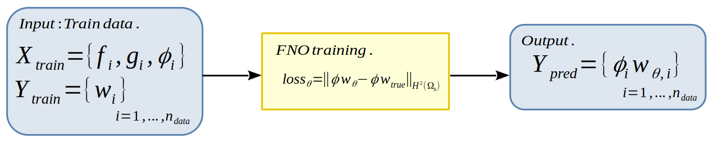
Here are the steps that will be performed to train the FNO (Figure 1):

We start by creating a dataset containing the level-set, source term and boundary condition collections, defined by

X_train = \{f_i,g_i,\phi_i\}_{i=1,\dots,n_{data}}.

Note that we can also consider the problem as homogeneous, in which case X_train will only be generated from \(f\) and \(\phi\). We may also wish to fix the geometry, in which case the training sample X_train will not contain the \(\phi\) term.

We can then solve these \(n_{data}\) problems using the \(\phi\)-FEM method, where the solution to each of them is defined by \(u=\phi w\). We then define the training sample

\[Y_train=\{w_i\}_{i=1,\dots,n_{data}}\]

where \(u_i = \phi_i w_i\) is the solution associated to the i-th problem of the X_train sample, i.e. solution of

\[\left\{\begin{aligned} -\Delta (\phi_i w_i)&=f_i, \; &&\text{on } \Omega, \\ u_i&=g_i, \; &&\text{in } \Gamma. \end{aligned}\right.\]

Note that in practice, we have enriched the data by increasing the number of channels in the X_train sample. In fact, for each problem \(i\), we add to the sample the primitives of \(f_i\) according to x and y, as well as the second primitives according to xx and yy. The X_train sample is then of size \((n_{data},ni,nj,nk)\) with \(nk=7\) the number of channels if we consider the 3 collections. The Y_train sample is of size \((n_{data},ni,nj,1)\).

At this moment, we have the (X_train,Y_train) pair that will enable us to train our FNO. More precisely, we’re looking to minimize a loss function on the model’s \(\theta\) parameters by using gradient descent. We’ll choose the following loss function:

loss_\theta = loss_\theta^{(0)} + loss_\theta^{(1)} + loss_\theta^{(2)}

with

\[\begin{aligned} loss_\theta^{(0)} &= \frac{1}{n_{data}}\sum_{i=1}^{n_{data}} mse(\phi_iw_i-\phi_iw_{\theta,i}) \\ loss_\theta^{(1)} &= \frac{1}{n_{data}}\sum_{i=1}^{n_{data}} mse(\nabla_x(\phi_iw_i)-\nabla_x(\phi_iw_{\theta,i}))+mse(\nabla_y(\phi_iw_i)-\nabla_y(\phi_iw_{\theta,i})) \\ loss_\theta^{(2)} &= \frac{1}{n_{data}}\sum_{i=1}^{n_{data}} mse(\nabla_{xx}(\phi_iw_i)-\nabla_{xx}(\phi_iw_{\theta,i})) + mse(\nabla_{yy}(\phi_iw_i)-\nabla_{yy}(\phi_iw_{\theta,i})) \end{aligned}\]

with \(w_i\) the \(\phi\)-FEM solution associated to the i-th problem considered (i.e. the i-th Y_train sample data), \(w_{\theta,i}\) the FNO prediction associated to the i-th problem, \(\phi_i\) the i-th level-set and mse the "Mean Square Error" function defined by

\[mse(A)=\frac{1}{ni}\frac{1}{nj}\sum_{i=0}^{ni-1}\sum_{j=0}^{nj-1}A_{i,j}^2.\]

Note that first and second derivatives according to x and y are calculated here by finite differences.

Figure 1. figure

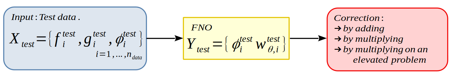
We can now proceed to the correction stage (Figure 2), where we consider a type of correction defined in Section "Presentation of the different correction methods considered" (correction by adding, correction by multiplying or correction by multiplying on an enhanced problem). We can then consider a new test sample X_test constructed in the same way as the training sample and defined by

\[X_test = \{f^{test}_i,g^{test}_i,\phi^{test}_i\}_{i=1,\dots,n_{test}}.\]

We will then provide this sample as input to the FNO in order to obtain its prediction \(w^{test}_{\theta,i}\) for each problem \(i\) of the test sample (where \(\theta\) corresponds to the parameters learned during training). We then construct \(u^{test}_{\theta_i}=\phi_i w^{test}_{\theta,i}\) which will be given as input to one of the correction solvers. We will then obtain what we call the corrected solution.

Figure 2. figure