Architecture of the FNO
The following figure (Figure 1) describes the FNO architecture in detail:
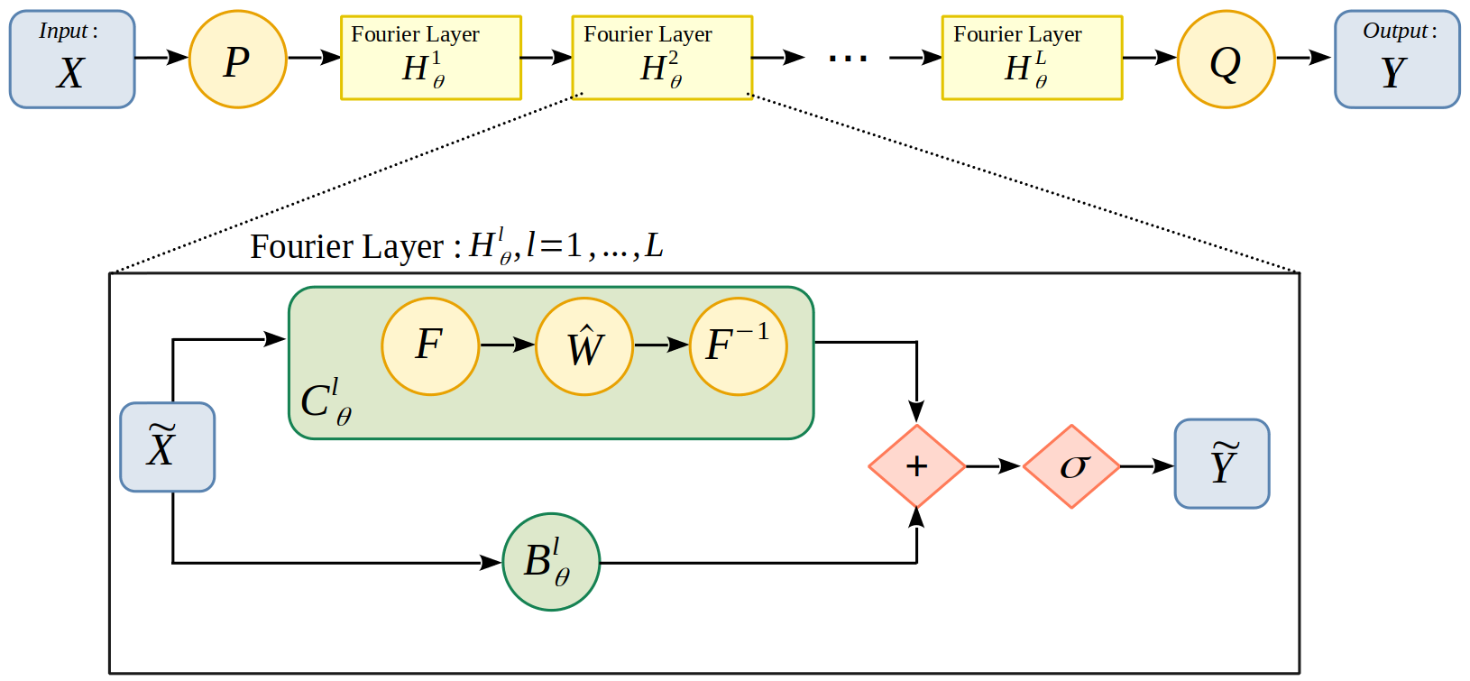
The architecture of the FNO is as follows:
We will now describe the composition of the Figure 1 in a little more detail :
-
We start with input X of shape (batch_size, height, width, nb_channels) with batch_size the number of images to be processed at the same time, height and width the dimensions of the images and nb_channels the number of channels. Simplify by (bs,ni,nj,nk).
-
We perform a \(P\) transformation in order to move to a space with more channels. This step enables the network to build a sufficiently rich representation of the data. For example, a Dense layer (also known as fully-connected) can be used.
-
We then apply \(L\) Fourier layers, noted \(\mathcal{H}_\theta^l,\; l=1,\dots,L\), whose specifications will be detailed in Section "Fourier Layer structure".
-
We then return to the target dimension by performing a \(Q\) transformation. In our case, the number of output channels is 1.
-
We then obtain the output of the \(Y\) model of shape (bs,ni,nj,1).
|
Note that the \(P\) and \(Q\) layers are in fact fully-connected multi-layer perceptrons, which means that they perform local transformations at each point, and therefore do not depend on the mesh resolution considered. Fourier layers are also independent of mesh resolution. Indeed, as we learn in Fourier space, the value of the Fourier modes does not depend on the mesh resolution. We deduce that the entire FNO does not depend on the mesh resolution. |