Some details on the convolution sub-layer

In this section, we will specify some details for the convolution layer.

1. Border issues

Let \(W=\mathcal{F}^{-1}(\hat{W})\), we have :

\[\mathcal{C}_\theta^l(\tilde{X})=\mathcal{F}^{-1}\left(\mathcal{F}(X)\cdot\hat{W}\right)=\tilde{X}\star W\]

with

\[(\tilde{X}\star W)_{ij}=\sum_{i'j'}\tilde{X}_{i-i'[ni],j-j'[nj]}W_{i'j'}\]

In other words, multiplying in Fourier space is equivalent to performing a \(\star\) circular convolution in real space.

These modulo operations are only natural for periodic images, which is not our case. The discontinuity that appears when we periodize the image causes oscillations on the edges of the filtered images. To limit this problem, we will apply a padding on the image which is the fact to extend the images by adding pixels all around, before performing the convolution. After the convolution, we restrict the image to partially erase the oscillations.

2. FFT

To speed up computations, we will use the FFT (Fast Fourier Transform). The FFT is a fast algorithm to compute the DFT. It is recursive : The transformation of a signal of size \(N\) is make from the decomposition of two sub-signals of size \(N/2\). The complexity of the FFT is \(N\log(N)\) whereas the natural algorithm, which is a matrix multiplication, has a complexity of \(N^2\).

3. Real DFT

In reality, we’ll be using a specific implementation of FFT, called RFFT (Real Fast Fourier Transform). In fact, for \(\mathcal{F}^{-1}(A)\) to be real if \(A\) is a complex-valued matrix, it is necessary that A respects the Hermitian symmetry:

\[A_{i,nj-(j+1)} = \bar{A}_{i,j}\]

In our case, we want \(\mathcal{C}_\theta^l(X)\) to be a real image, so \(\mathcal{F}(X)\cdot\hat{W}\) must verify Hermitian-symmetry.

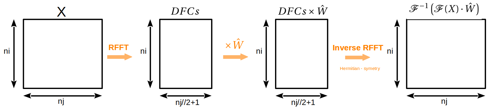
To do this, we only need to collect half of the Discrete Fourier Coefficients (DFC) and the other half will be deduced by Hermitian symmetry. More precisely, using the specific RFFT implementation, the DFCs are stored in a matrix of size \((ni,nj//2+1)\). Multiplication can then be performed by the \(\hat{W}\) kernel, and when the inverse RFFT is performed, the DFCs will be automatically symmetrized. So the Hermitian symmetry of \(\mathcal{F}(X)\cdot\hat{W}\) is verified and \(\mathcal{C}_\theta^l(X)\) is indeed a real image.

To simplify, let’s assume nk=1. Here is a diagram describing this idea:

Figure 1. figure

In fact, we can check that \(\mathcal{F}(X)\) satisfies Hermitian symmetry immediately.

4. Low pass filter

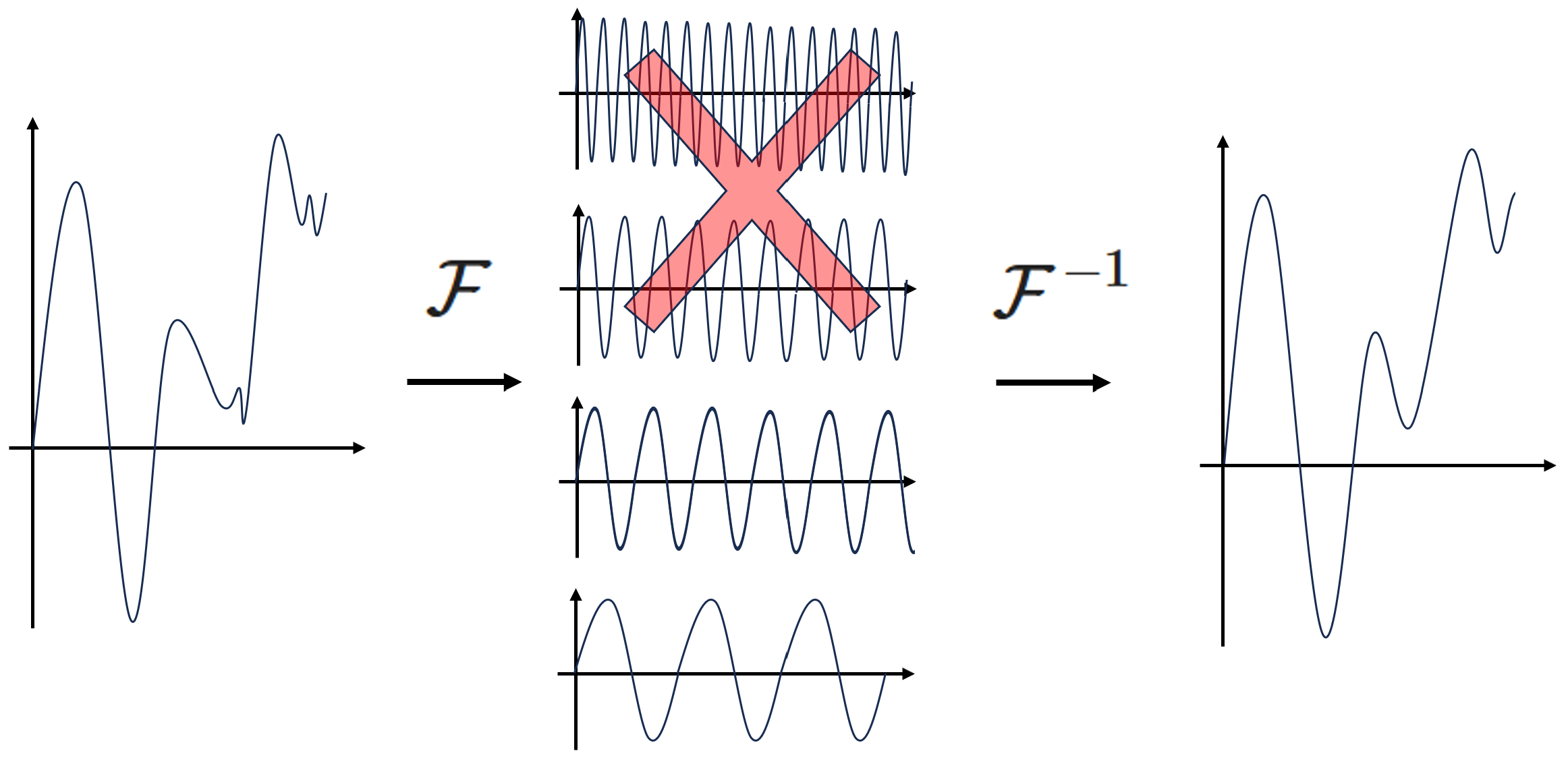
When we perform a DFT on an image, the DFCs related to high frequencies are in practice very low. This is why we can easily filter an image by ignoring these high frequencies, i.e. by truncating the high Fourier modes. In fact, eliminating the higher Fourier modes enables a kind of regularization that helps the generalization. So, in practice, it’s sufficient to keep only the DFCs corresponding to low frequencies. Typically, for images of resolution \(32\times 32\) to \(128\times 128\), we can keep only the \(20\times 20\) DFCs associated to low frequencies.

Here is a representation of this idea in 1D :

Figure 2. figure

5. Global aspect of the FNO

Classical Convolutional Neural Networks (CNN) use very small kernels (typically \(3\times 3\)). This operation only has a local effect, and it’s the sequence of many convolutions that produces more global effects.

In addition, CNNs often use max or mean-pooling layers, which process the image on several scales. Max-pooling (respectively mean-pooling) consists in slicing the image into small pieces of size \(n\times n\), then choosing the pixel with the highest value (respectively the average of the pixels) in each of the small pieces. In most cases, \(n=2\) is used, which divides the number of pixels by 4.

The FNO, on the other hand, uses a \(\hat{W}\) frequency kernel and \(W=\mathcal{F}^{-1}(\hat{W})\) has full support. For this reason, the effect is immediately non-local. As a result, we can use less layers and we don’t need to use a pooling layer.