General presentation of the \(\phi\)-FEM method

In this section, we will present the \(\phi\)-FEM method. We consider the case of the Poisson problem with homogeneous Dirichlet boundary conditions \cite{duprez_phi-fem_2020}.

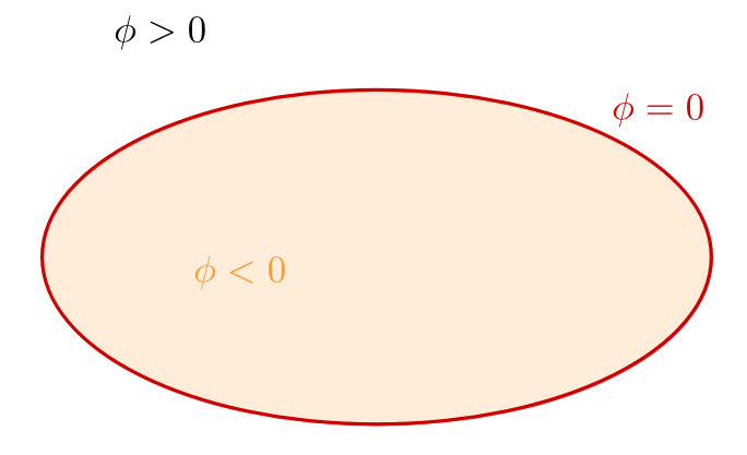
\[\left\{ \begin{aligned} -\Delta u &= f, \; &&\text{in } \; \Omega, \\ u&=g, \; &&\text{on } \; \partial\Omega, \end{aligned} \right. \label{eq.Poisson}\]

where the domain \(\Omega\) and its boundary \(\Gamma\) are given by a level-set function \(\phi\) such that

\[\Omega=\{\phi < 0\} \quad \text{and} \quad \Gamma=\{\phi = 0\}.\]

Figure 1. Definition of the level-set function.

For more details on mesh assumptions, convergence results and finite element matrix condition number, please refer to \cite{duprez_phi-fem_2020}. \(\phi\)-FEM schemes for the Poisson problem with Neumann or mixed (Dirichlet and Neumann) conditions are presented in \cite{duprez_new_2023,cotin_phi-fem_nodate}. The \(\phi\)-FEM scheme can also be found for other PDEs, including linear elasticity \cite[Chapter~2]{cotin_phi-fem_nodate}, the heat equation \cite[Chapter~5]{cotin_phi-fem_nodate} and the Stokes problem \cite{duprez_phi-fem_2023}.

Example. If \(\; \Omega\) is a circle of center \(A\) of coordinates \((x_A,y_A)\) and radius \(r\), a level-set function can be defined by

\[\phi(x,y)=-r^2+(x-x_A)^2+(y-y_A)^2.\]

If \(\; \Omega\) is an ellipse with center \(A\) of coordinates \((x_A,y_A)\) and parameters \((a,b)\), a level-set function can be defined by

\[\phi(x,y)=-1+\frac{(x-x_A)^2}{a^2}+\frac{(y-y_A)^2}{b^2}.\]

We assume that \(\Omega\) is inside a domain \(\mathcal{O}\) and we introduce a simple quasi-uniform mesh \(\mathcal{T}_h^\mathcal{O}\) on \(\mathcal{O}\) (Figure 2).

We introduce now an approximation \(\phi_h\in V_{h,\mathcal{O}}^{(l)}\) of \(\phi\) given by \(\phi_h=I_{h,\mathcal{O}}^{(l)}(\phi)\) where \(I_{h,\mathcal{O}}^{(l)}\) is the standard Lagrange interpolation operator on

\[V_{h,\mathcal{O}}^{(l)}=\left\{v_h\in H^1(\mathcal{O}):v_{h|_T}\in\mathbb{P}_l(T) \; \forall T\in\mathcal{T}_h^\mathcal{O}\right\}\]

and we denote by \(\Gamma_h=\{\phi_h=0\}\), the approximate boundary of \(\Gamma\) (Figure 3).

We will consider \(\mathcal{T}_h\) a sub-mesh of \(\mathcal{T}_h^\mathcal{O}\) obtained by removing the elements located entirely outside \(\Omega\) (Figure 3). To be more specific, \(\mathcal{T}_h\) is defined by

\[\mathcal{T}_h=\left\{T\in \mathcal{T}_h^\mathcal{O}:T\cap\{\phi_h<0\}\ne\emptyset\right\}.\]

We denote by \(\Omega_h\) the domain covered by the \(\mathcal{T}_h\) mesh (\(\Omega_h\) will be slightly larger than \(\Omega\)) and \(\partial\Omega_h\) its boundary (Figure 3). The domain \(\Omega_h\) is defined by

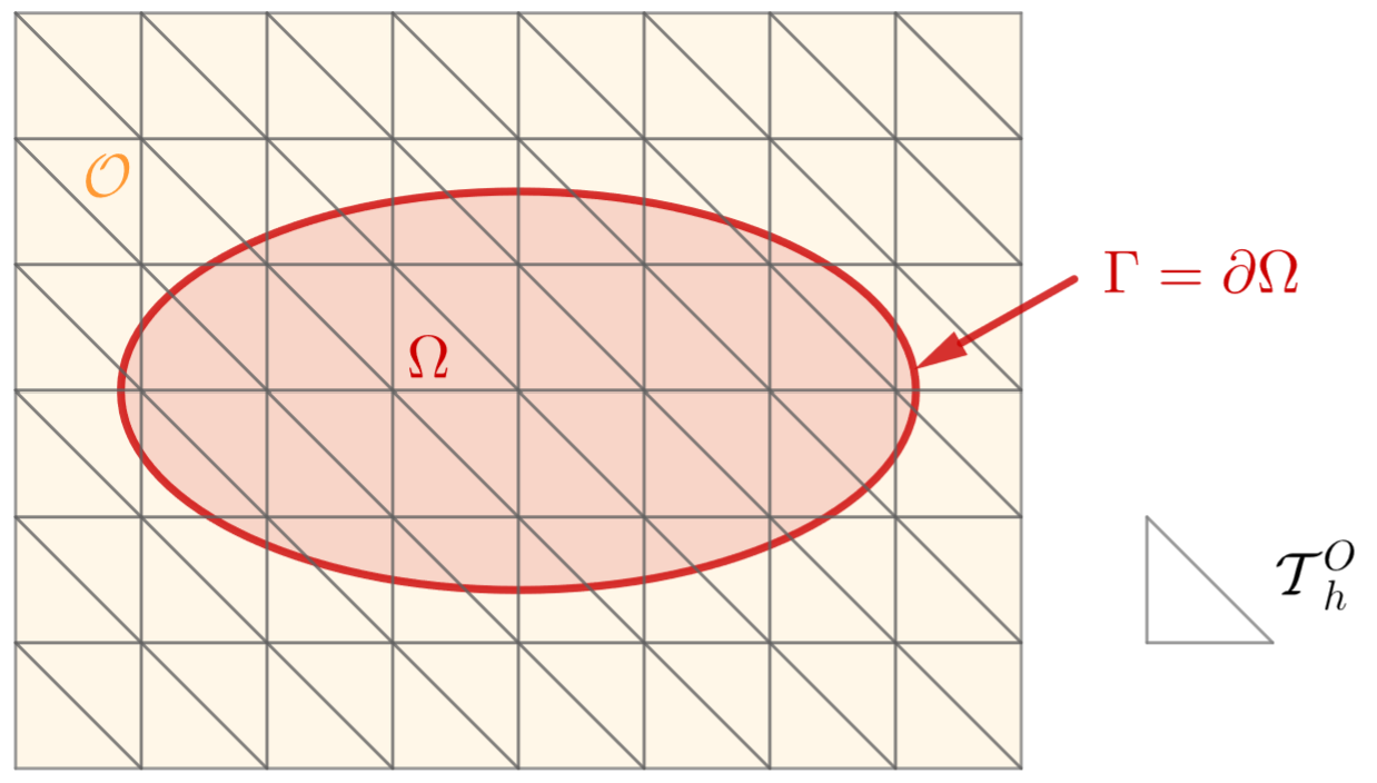
\[\Omega_h=\left(\cup_{T\in\mathcal{T}_h}T\right)^O.\]

Figure 2. Fictitious domain.

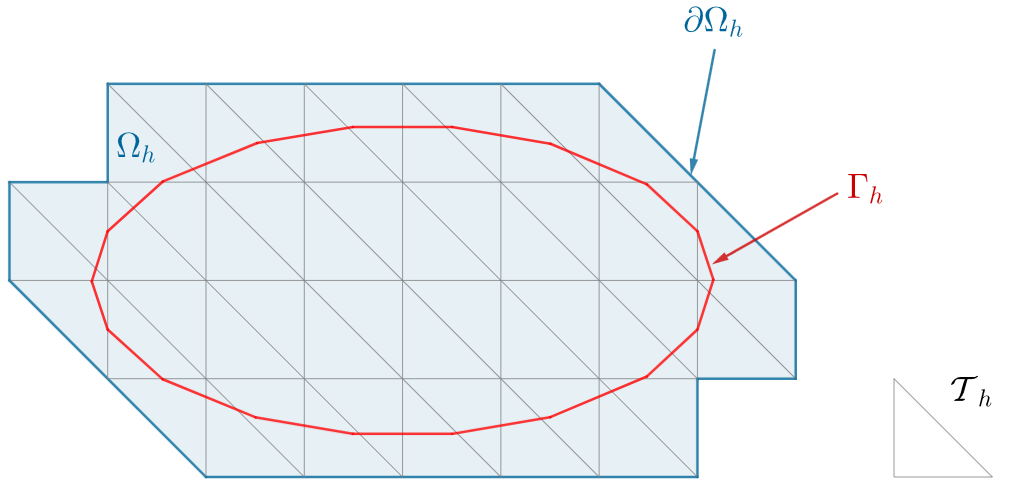
Figure 3. Domain considered.

Now, we can introduce \(\mathcal{T}_h^\Gamma\subset \mathcal{T}_h\) (Figure 4) which contains the mesh elements cut by the approximate boundary \(\Gamma_h = \{\phi_h=0\}\), i.e.

\[\mathcal{T}_h^\Gamma=\left\{T\in \mathcal{T}_h:T\cap\Gamma_h\ne\emptyset\right\},\]

and \(\mathcal{F}_h^\Gamma\) (Figure 5) which collects the interior facets of the mesh \(\mathcal{T}_h\) either cut by \(\Gamma_h\) or belonging to a cut mesh element

\[\mathcal{F}_h^\Gamma=\left\{E\;(\text{an internal facet of } \mathcal{T}_h) \text{ such that } \exists T\in \mathcal{T}_h:T\cap\Gamma_h\ne\emptyset \text{ and } E\in\partial T\right\}.\]

We denote by \(\Omega_h^\Gamma\) the domain covered by the \(\mathcal{T}_h^\Gamma\) mesh (Figure 4) and also defined by

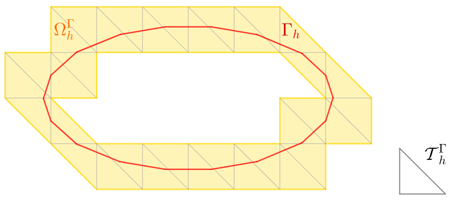
\[\Omega_h^\Gamma=\left(\cup_{T\in\mathcal{T}_h^\Gamma}T\right)^O.\]

Figure 4. Boundary cells.

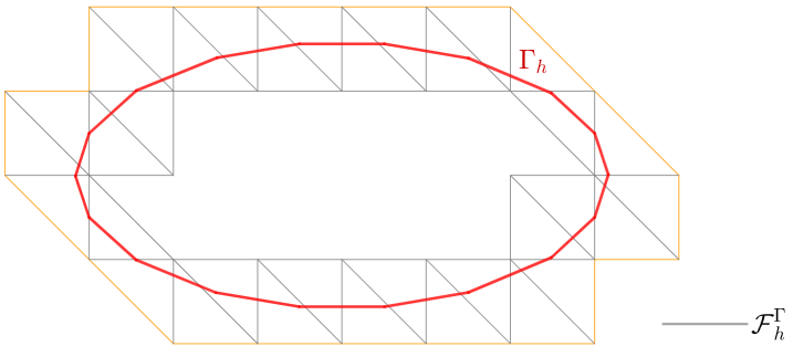
Figure 5. Boundary edges.